Improving Speed and Quality of Image Generation
Welcome to the third installment of our series on the Diffusers library. In this post, we’ll explore strategies to enhance both the inference speed and the quality of generated images. Thus, we will improve the techniques discussed in our previous article, also, we will also use new ones.
Note on Best Practices
Before we dive into the technical details, it’s important to note that this post does not adhere to all best practices typically recommended for machine learning projects. Specifically, we are not utilizing dataset versioning, tracking tools like MLflow, or hyperparameter optimization frameworks such as Optuna. These practices are essential for a robust ML workflow and will be addressed in future posts, though not immediately. The focus of this tutorial is to present a simplified workflow that is easier to follow and understand.
Data Analysis: The Crucial First Step#
Analyzing the data is a critical first step in improving image generation quality.
Understanding Data Distribution#
Let's start by examining the distribution of our dataset. This will help us identify any imbalances or anomalies in the data.
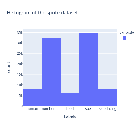
Currently, our dataset is not balanced. Balancing it will enhance the model's performance by improving its ability to generalize and produce more accurate results. We can do it with the following addition in our training notebook:
dataset = SpritesDataset(
    "./dlai_lib/sprites_1788_16x16.npy",
    "./dlai_lib/sprite_labels_nc_1788_16x16.npy",
    null_context=False
)

# Create dataset sampler to compensate the unbalanced dataset
labels = dataset.slabels.argmax(axis=1)
u_labels, class_counts = np.unique(labels, return_counts=True)
class_weights = 1 - class_counts / class_counts.sum()
sample_weights = tuple(class_weights[label] for label in labels)
num_samples = ceil(len(labels)/batch_size) * batch_size # num_samples is a multiple of batch_size to avoid recompiling

dataset_sampler = WeightedRandomSampler(weights=sample_weights, num_samples=num_samples, replacement=True)

dataloader = DataLoader(
    dataset, sampler=dataset_sampler, batch_size=batch_size, num_workers=1, pin_memory=True
)
In this approach, we calculate weights for each sample in our dataset and use a random data sampler to select samples according to these weights. As a result, samples from the least represented classes are selected more frequently than those from the more prevalent classes.
Despite the non-human class being one of the most prevalent in our dataset, the model struggles to generate anything beyond indistinct blobs, indicating that there may be underlying issues with the data itself.
Analyzing Non-Human Class#
A major challenge for our model is the non-human class, which frequently includes poorly representative images. To illustrate this issue, let’s first examine the original non-human images:

As observed, some examples are of poor quality and resemble the non-human outputs produced by our model. To address this, we will investigate and develop a function to automatically detect such problematic samples in the database, as reviewing over 80,000 samples manually is not feasible.
def detect_wrong_images(image: np.ndarray, number_of_white: int = 26) -> bool:
    """Function to detect if an image is a wrong one and should be excluded from training.

    Parameters
    ----------
    image : np.ndarray
        the image in RGB with shape [width, heigh, channel]
    number_of_white : int, optional
        the number of white pixel a function must have to be considered valid, by default 26

    Returns
    -------
    bool
        True if it is a wrong image for generation and False if it is a good one.
    """

    wrong_image = False
    # Note white is (255, 255, 255) hence the sum is 765
    # White background so a minimum of pixel should be white
    wrong_image |= np.sum(image.sum(axis=-1) == 765) < number_of_white

    # 4 corners must be white
    wrong_image |= image[0, 0].sum() != 765
    wrong_image |= image[-1, 0].sum() != 765
    wrong_image |= image[0, -1].sum() != 765
    wrong_image |= image[-1, -1].sum() != 765

    return wrong_image
The purpose of this function is straightforward: good images should have all corners white and a significant portion of the pixels should be white, as we expect white backgrounds. While this approach is sufficient for a relatively simple dataset, real-world datasets will require additional checks, such as for blurriness and color palette constraints.
If we plot some bad samples we obtain this:
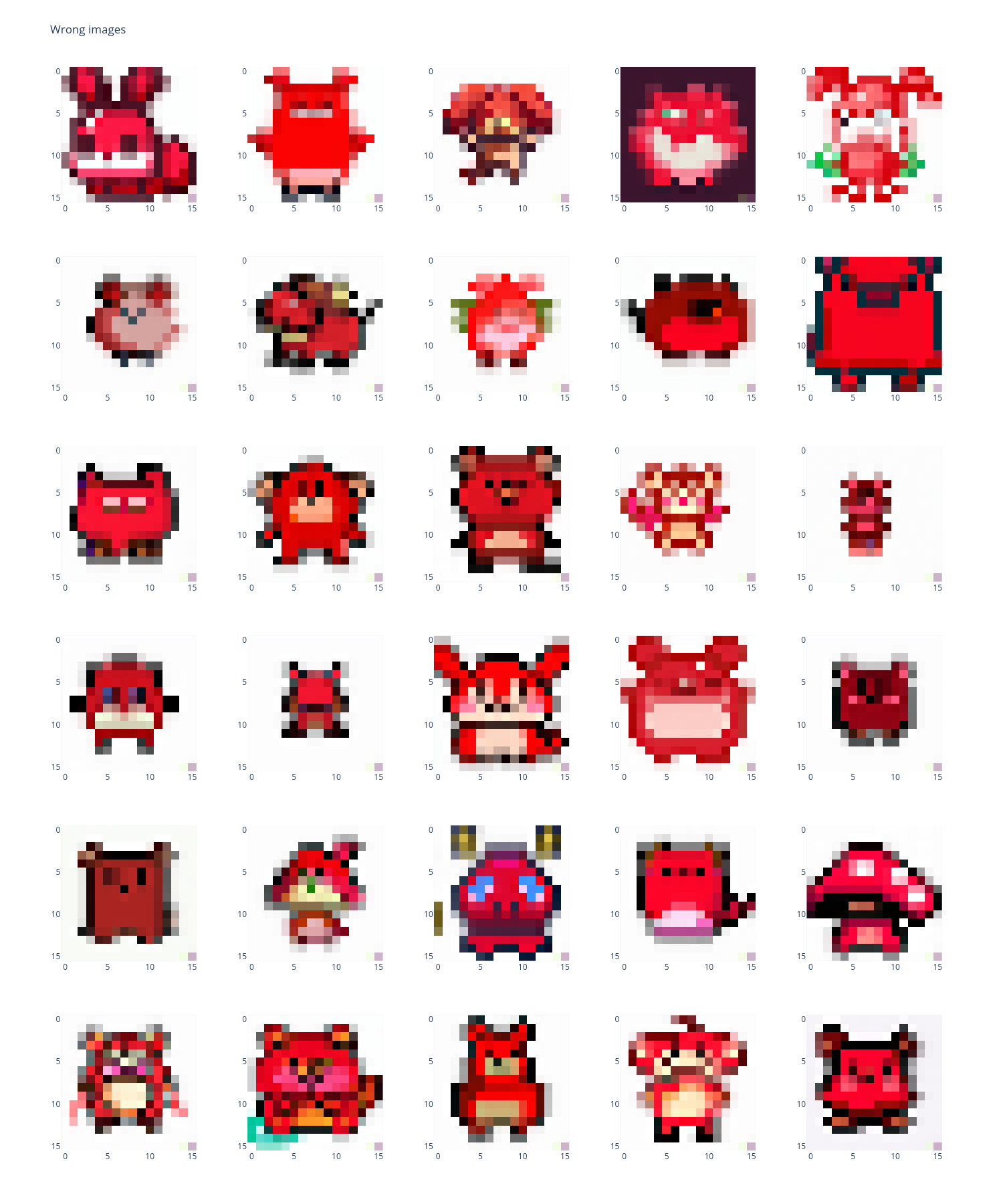
Using this approach, we identified and removed 30,000 problematic samples from our dataset, effectively capturing the key issues for the non-human class.
And if we show the 30 non-human examples of our new dataset, we obtain this:

Applying this function to refine our dataset can accelerate model training and significantly improve results. However, you might still find that the quality of the generated images is insufficient and the generation process is too slow.
I created a custom dataset to enable this filtering with clean_version=True parameter.
Note
For a detailed explanation of this process, please refer to the dedicated notebook here: https://github.com/vroger11/diffusers-tutorials/tree/main/tutorials/03-dataset_analysis.ipynb
Enhancements in Network Design#
Typically, people might think that adding more layers and parameters will improve the model. While this can be true in some cases, it's not the complete solution and often leads to inefficient models. In the following subsections, we will explore techniques to enhance the results and inference speed.
Conditional Network Warm-Up#
To enforce the conditioned result concordance we use a warm-up strategy for the conditional network. But, this induce overfitting of the UNet over the ground truth. To tackle this problem, after freezing the parameters of the conditional network, we apply random masking of labels (context) using a Bernoulli distribution. This approach stabilizes the training process and helps prevent the UNet from overfitting to the conditional network.
I’ve chosen an arbitrary warm-up value of 80 for demonstration purposes in this tutorial. This may not be the optimal value for all scenarios. In real-world applications, it is advisable to monitor model performance and adjust the warm-up step accordingly to determine the best time to freeze the conditional network.
These adjustments are implemented by incorporating the following two conditions into our training loop:
if epoch >= warmup:
    warmup_done = True
    # freeze all layers of the embedding network
    for param in emb_net.parameters():
        param.requires_grad = False
if warmup_done:
    # randomly mask out labels (context)
    context_mask = torch.bernoulli(torch.zeros(labels.shape[0]) + 0.95).to(unet.device)
    labels = labels * context_mask.unsqueeze(-1)
Network Architecture Improvements#
UNet Enhancements#
Adding both a down block and an up block to the UNet architecture has proven effective. My experiments showed that omitting these blocks led to a decline in the quality of generated images.
Therefore, we modify our UNet like follows:
unet = UNet2DConditionModel(
    encoder_hid_dim=class_emb_size,
    sample_size=16,
    in_channels=3,
    out_channels=3,
    layers_per_block=2,
    block_out_channels=(64, 128, 256),
    down_block_types=("DownBlock2D", "DownBlock2D", "CrossAttnDownBlock2D"),  # One more down block
    up_block_types=("CrossAttnUpBlock2D", "UpBlock2D", "UpBlock2D"),  # One more up block
)
Conditional Network Bottleneck#
Implementing a bottleneck in the conditional network enforces better embedding quality, which in turn enhances overall performance.
As a result, our embedding network becomes:
emb_net = CustomSequential(
    nn.Linear(num_classes, class_emb_size//2), # bottleneck to force better embeddings quality
    nn.GELU(),
    nn.Linear(class_emb_size//2, class_emb_size),
    UnsqueezeLayer(dim=1),
)
Regularization Techniques#
Regularization is essential for improving model generalization and preventing overfitting:
Dropout#
We apply dropout to both the UNet and the embedding network to reduce overfitting and improve model robustness.
This results in the following modifications:
emb_net = CustomSequential(
    nn.Linear(num_classes, class_emb_size//2),
    nn.Dropout(0.1), # add of dropout to regularize the model
    nn.GELU(),
    nn.Linear(class_emb_size//2, class_emb_size),
    UnsqueezeLayer(dim=1),
)

# Define the UNet model
unet = UNet2DConditionModel(
    encoder_hid_dim=class_emb_size,
    sample_size=16,
    in_channels=3,
    out_channels=3,
    layers_per_block=2,
    block_out_channels=(64, 128, 256),
    down_block_types=("DownBlock2D", "DownBlock2D", "CrossAttnDownBlock2D"),
    up_block_types=("CrossAttnUpBlock2D", "UpBlock2D", "UpBlock2D"),
    dropout=0.2, # add of dropout to regularize the model
)
Note that we avoid applying Dropout to the output of our embedding network to prevent issues, such as optimizing zeroed embedding values from Dropout, which can affect the attention mechanism in our UNet.
AdamW Optimizer#
We use the AdamW optimizer, which incorporates weight decay. This technique aids in better regularization by penalizing large weights.
So set this up, we have to change an import:
from torch.optim import AdamW
Also change the optimizer creation and using a weight_decay, here I chose an arbitrary value that works well in most cases but deserve to be chosen more carefully if you have the computations capacities:
optimizer = AdamW(chain(unet.parameters(), emb_net.parameters()), lr=lr, weight_decay=1e-4)
Scheduler and Loss Function Adjustments#
DDIM vs. DDPM#
DDIM (Denoising Diffusion Implicit Models) offers several advantages over DDPM (Denoising Diffusion Probabilistic Models). Unlike DDPM, which relies on a Markov chain to sequentially denoise samples, DDIM bypasses the explicit Markov process by using a non-Markovian approach that allows for fewer diffusion steps. This results in faster and more efficient sampling while maintaining or even improving the quality of the generated images.
Switching from DDPM to DDIM is straightforward; we simply need to start by replacing the noise scheduler creation:
# Use of DDIMScheduler instead of DDPMScheduler
noise_scheduler = DDIMScheduler(num_train_timesteps=1000)
Since the API of the DDIMScheduler is similar to that of the DDPMScheduler, there's no need to modify the code related to the noise_scheduler.
However, we do need to rewrite our pipeline, though it closely resembles our custom DDPMPipeline.
class ConditionalDDIMPipeline(DDIMPipeline):
    def __init__(
        self, unet: UNet2DConditionModel, class_net: CustomSequential, scheduler: DDIMScheduler
    ) -> None:
        super().__init__(unet=unet, scheduler=scheduler)
        self.class_net = class_net
        self.class_net.eval()
        self.register_modules(class_net=class_net)
        self.unet.eval()

    @torch.no_grad()
    def __call__(
        self,
        class_label: list[list[float]],
        generator: Optional[Union[torch.Generator, List[torch.Generator]]] = None,
        eta: float = 0.0,
        num_inference_steps: int = 1000,
        use_clipped_model_output: Optional[bool] = None,
        output_type: Optional[str] = "pil",
        return_dict: bool = True,
    ) -> Union[ImagePipelineOutput, Tuple]:
        r"""
        The call function to the pipeline for generation.

        Args:
            class_label (list[list[float]]):
                list of one-hot examples. len(class_label) represents the number of examples to generate.
            generator (`torch.Generator`, *optional*):
                A [`torch.Generator`](https://pytorch.org/docs/stable/generated/torch.Generator.html) to make
                generation deterministic.
            eta (`float`, *optional*, defaults to 0.0):
                Corresponds to parameter eta (η) from the [DDIM](https://arxiv.org/abs/2010.02502) paper. Only applies
                to the [`~schedulers.DDIMScheduler`], and is ignored in other schedulers. A value of `0` corresponds to
                DDIM and `1` corresponds to DDPM.
            num_inference_steps (`int`, *optional*, defaults to 1000):
                The number of denoising steps. More denoising steps usually lead to a higher quality image at the
                expense of slower inference.
            use_clipped_model_output (`bool`, *optional*, defaults to `None`):
                If `True` or `False`, see documentation for [`DDIMScheduler.step`]. If `None`, nothing is passed
                downstream to the scheduler (use `None` for schedulers which don't support this argument).
            output_type (`str`, *optional*, defaults to `"pil"`):
                The output format of the generated image. Choose between `PIL.Image` or `np.array`.
            return_dict (`bool`, *optional*, defaults to `True`):
                Whether or not to return a [`~pipelines.ImagePipelineOutput`] instead of a plain tuple.

        Returns:
            [`~pipelines.ImagePipelineOutput`] or `tuple`:
                If `return_dict` is `True`, [`~pipelines.ImagePipelineOutput`] is returned, otherwise a `tuple` is
                returned where the first element is a list with the generated images
        """
        batch_size = len(class_label)
        # Sample gaussian noise to begin loop
        if isinstance(self.unet.config.sample_size, int):
            image_shape = (
                batch_size,
                self.unet.config.in_channels,
                self.unet.config.sample_size,
                self.unet.config.sample_size,
            )
        else:
            image_shape = (batch_size, self.unet.config.in_channels, *self.unet.config.sample_size)

        image = randn_tensor(image_shape, generator=generator, device=self._execution_device, dtype=self.unet.dtype)

        # get encoded ground truth
        labels = torch.tensor(class_label, device=self.device)
        with autocast(str(self.unet.device)):
            enc_labels = self.class_net(labels)

            # set step values
            self.scheduler.set_timesteps(num_inference_steps)

            for t in self.progress_bar(self.scheduler.timesteps):
                # 1. predict noise model_output
                model_output = self.unet(image, t, enc_labels, class_labels=labels, return_dict=False)[
                    0
                ]

                # 2. predict previous mean of image x_t-1 and add variance depending on eta
                # eta corresponds to η in paper and should be between [0, 1]
                # do x_t -> x_t-1
                image = self.scheduler.step(
                    model_output, t, image, eta=eta, use_clipped_model_output=use_clipped_model_output, generator=generator
                ).prev_sample

        image = (image / 2 + 0.5).clamp(0, 1)
        image = image.cpu().permute(0, 2, 3, 1).numpy()

        if output_type == "pil":
            image = self.numpy_to_pil(image)

        if not return_dict:
            return (image,)

        return ImagePipelineOutput(images=image)
We modified the inheritance and added the eta parameter to ensure compatibility with the DDPMScheduler. With this scheduler, I was able to generate high-quality samples in just 10 steps, instead of 100, significantly improving the inference speed of our final model by over 10 times, as we also employ a non-Markovian approach.
Loss Function#
We switch from L2 loss to L1 loss. L1 loss, or Mean Absolute Error (MAE), is less sensitive to outliers compared to L2 loss (Mean Squared Error), making it more robust and stable during training. This robustness helps in generating clearer and more visually coherent images by reducing the influence of extreme values and ensuring stable gradient updates.
In our previous code, this requires modifying the loss function computation:
# Compute l1 loss instead of mse, it provides better robustness to noises
# which is suited for diffusion models, but the cost is slower training
loss = torch.nn.functional.l1_loss(predicted_noise, noise)
Training Enhancements#
Increased Epochs#
With the aforementioned modifications, we have increased the number of training epochs to 100. This ensures that the model is trained thoroughly and can better leverage our previous modifications.
Torch Compile#
To speed up training we already used mixed precision. But, we can go further using torch.compile. This results in a 30% reduction in training time. Note that torch.compile was not used for the final pipeline, as we required a single forward pass for evaluation. However, torch.compile offers significant efficiency benefits for serving models.
To compile our networks, we need to add the following lines:
# compile networks for faster inferences even for training
unet = torch.compile(unet, fullgraph=True)
emb_net = torch.compile(emb_net, fullgraph=True)
For those interested in achieving even faster results through techniques like quantization and distillation, I recommend checking out the Hugging Face tutorial on fast diffusion.
Final result#
Before presenting the final results, I’d like to set some realistic expectations. With the current dataset (excluding poor examples), we can expect good results. However, keep in mind that we are working with only five categories in our ground truth, and the examples within each category are quite heterogeneous. As a result, while the model will learn to distinguish between the categories, it won't capture the finer "sub-categories," limiting our control over them. This lack of homogeneity within categories leaves room for the ground truth to be more easily mixed.
Now, let's take a look at some samples from each class:

As you can see, the images appear quite polished, but many of the generated results are nearly identical to some training examples. You might notice subtle differences between the originals and generated samples (especially with small details like for flames). To better control the subcategories, we could enhance the ground truth by subdividing the existing categories. This task is labor-intensive if done manually. A more efficient approach is to automate it by applying algorithms like k-means in the encoded space of our UNet over the training samples and assigning names to the resulting categories. This would make the mixing of categories more meaningful and allow for more flexibility in tweaking the embeddings.
However, since I need to set limits for this tutorial to avoid it becoming overly extensive, I’m marking this part as out of scope.
I hope this post helps and/or inspires some of you. If you have suggestions feel free to comment or reach me.
See you again, Vincent.